Distinctive rings in the 21 cm signal of the epoch of reionization
1er mars 2011
9 March 2011 — The epoch of reionization is the moment in the universe when the hydrogen gas, first essentially neutral, becomes ionized by the first UV and X-ray sources (stars and quasars). Astrophysicists hope to get information on the epoch of reionization from future observations of the 21 cm transition of neutral hydrogen, for which numerous projects are in development ((LOFAR, SKA, MWA..). However, it will be difficult to extract the cosmological signal from the raw data because of foreground sources, ionospheric refraction, or the instrumental contamination. The intensity of the foregrounds will be several orders of magnitude greater than that of the 21 cm signal. Any prediction about the properties of the signal is therefore useful as a diagnostic to test systematics and foreground removal procedures. Such a prediction has been precisely done by researchers of the Paris Observatory (LERMA). Using numerical simulations, they emphasized the existence of a ring-shaped signal around the first light sources.
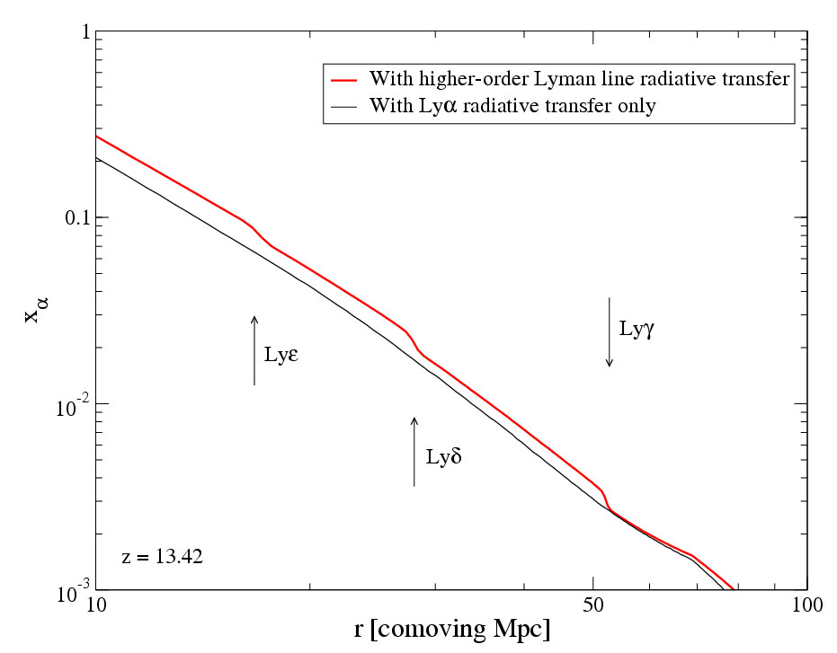
As a result, any source emitting in the UV band is surrounded by a series of concentric shells, so-called Lyman horizons, that photons emitted in given frequency bands cannot overtake. Therefore, the Lyman-alpha flux radial profile around UV sources shows characteristic discontinuities at distances where the emitted photons reach the different Lyman-series lines (Figure 1).
Figure 1 : Profil radial du coefficient de couplage pour l’excitation par Lyman-alpha, x_alpha, à z=13.42, autour de la première source apparaissant dans une simulation de 140 Mpc de taille (cette taille correspond à la taille mesurée aujourd’hui, en soustrayant l’expansion, on la dit "comobile"). La courbe rouge est le profil correct, alors que la courbe noire est le résultat d’une simulation négligeant l’apport des photons Lyman-alpha issus des raies supérieures de la série de Lyman. De nettes discontinuités s’observent aux positions correspondant aux horizons Lyman-gamma, Lyman-delta et Lyman-epsilon, dont les positions prédites sont indiquées par des flèches.
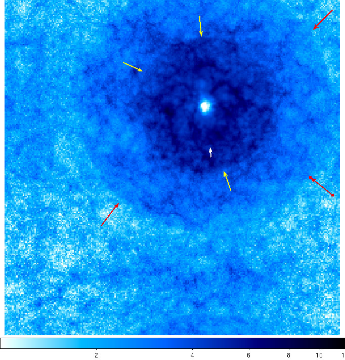
Because of the Wouthuysen-Field effect, this translates into a similar profile for the differential brightness temperature of the 21 cm signal. On maps of that signal, Lyman horizons are marked as concentric, perfectly spherical rings around the sources (Figure 2).
Figure 2 : Carte de la quantité Delta T_b r2 à z = 13.42, où Delta T_b est la température différentielle (déviation par rapport au fond diffus cosmologique) de brillance du signal à 21 cm et r la distance au centre de la source. L’échelle de couleur est logarithmique et en unités arbitraires. Les horizons Lyman-epsilon, Lyman-delta et Lyman-gamma sont marqués de flèches blanche, jaunes et rouges respectivement. L’image fait 140 Mpc comobiles de côté et a une épaisseur de 2.8 Mpc comobiles. La source de rayonnement se trouve au centre d’une bulle d’hydrogène ionisé (tache blanche centrale).
Unfortunately, other nearby sources, appearing progressively in the simulation, will also contribute to the Lyman-alpha background, making it more and more anisotropic. This will progressively wipe out the ring-shaped discontinuities. The LERMA team showed that rings are visible during a redshift interval Delta z 2 after the first light source lit up. Using a stacking technique (averaging the radial profiles of all the sources in the simulation), they are able to extend this interval to Delta z 4, i.e. from z=14 to z=10 approximately.
It is interesting to determine whether that predicted signature will be detectable by the planned Square Kilometre Array, a huge radiotelescope in development which will be considerably more sensitive than any other radio instrument. In order to do so, instrumental noise has been added to the predicted signal. Analysis shows that if the number of sources is sufficient, the profile averaging procedure allows individual fluctuations to be smoothed, and then Lyman horizons are still detectable (Figure 3).
Figure 3 : Gradient du profil radial du signal à 21 cm, à z=11.05, pour une simulation de 280 Mpc comobiles de côté. La courbe noire se réfère à la première source apparaissant dans la simulation, sans ajout de bruit instrumental. La courbe rouge se rapporte à la même source, mais après avoir ajouté du bruit. Quant à la courbe bleue, c’est celle du gradient du profil lorsque toutes les sources de la simulation ont été sommées ensemble. Cette méthode de moyenne est efficace, puisqu’elle permet de mettre en évidence les horizons Lyman-delta et Lyman-epsilon (pics du gradient, indiqués par des flèches), alors que ceux-ci ne sont pas détectables sur les profils individuels, bruités ou non.